Joining and shuffling very large datasets using Cloud Dataflow
Marián Dvorský
Software Engineer, Google Cloud Platform
Riju Kallivalappil
Software Engineer
Google Cloud Dataflow customers looking for better scalability, performance, and predictability of their batch pipelines have rapidly adopted Cloud Dataflow Shuffle (available in beta) to shuffle datasets big and small. Shuffle is the base data transformation that enables grouping and joining of datasets.
Over the past several months, we’ve shared many user stories that highlight the ways in which customers benefit from using Cloud Dataflow Shuffle, including:
- Less variability in pipeline execution times, allowing users to better plan their workflows
- Faster execution of
GroupByKeyandCoGroupByKeyoperations and of the overall Dataflow pipeline - Better handling of hot key situations, reduced resource consumption and execution times
Cloud Dataflow Shuffle at large scale
Consider a case in which you have to join two datasets by key. In our sample pipeline, we have two text files that we want to join in a left outer join and then save the results into a file. In a real production pipeline, one of the files might store user web session data and the other file might contain purchase records, and the result of the join might be purchase records enriched with user activity information. The pipeline is written in Scala, using the succinct Scala-based Scio API developed by Spotify. Spotify uses Cloud Dataflow at a volume of 80,000 Dataflow jobs per month and recently blogged about how Scio helps them with creating and maintaining their extensive data processing infrastructure comprised of thousands of distinct pipelines.Sample Cloud Dataflow pipeline written in Scio, a Scala-based API developed by Spotify
Here is the pipeline graph:
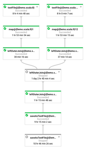
The leftOuterJoin() function in the above code snippet implements this join in Cloud Dataflow by applying a CoGroupByKey transform. When Dataflow encounters a CoGroupByKey, it tags records from either side of the join, flattens (merges) both datasets, and then runs a shuffle (grouping) operation on the merged dataset. After the shuffle, Dataflow provides an iterator over records with the same key so that your remaining pipeline code can process the joined data.
Joining two 1TB-size datasets took less than 20 minutes in this pipeline. But what happened when we increased the dataset size ten-fold, trying to join two 10TB datasets? The duration of the 10TB pipeline did increase, but it increased by less than 10x because Dataflow automatically sensed that there was more work to be done and it had exhausted the available resources to their maximum. In both pipeline runs, our pipeline’s resources were limited by 1000 1-vCPU workers (we set the worker maximum before launching the pipeline). Our 10Tx10T pipeline ran in ~90 minutes, or ~4.5 times longer than our 1Tx1T pipeline.
| Dataset Size | 1TB x 1TB | 10TB x 10TB |
| Duration of the pipeline | 19 minutes | 1 hour 33 minutes |
| Worker CPU usage | 129 | 1,468 |
| Shuffle GB-hours | 453 | 30,505 |
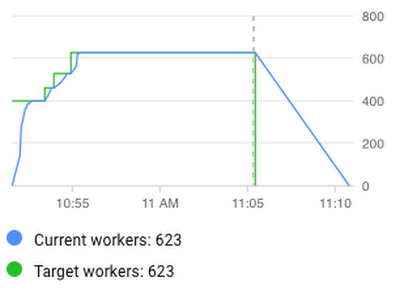
As you can see in the worker utilization charts, our 1TB x 1TB (1 terabyte of data joined with another TB of data) pipeline gradually increased the number of workers used in this process until it reached the limit of parallelization for this dataset at 623 workers (it never needed the full 1000 workers that we allocated for this job). Our 10-times larger pipeline went beyond the 623 workers and used all available resources to minimize the execution time. The Dataflow feature that enabled this efficient and performance-optimized usage of resources is called autoscaling.

Though we use it as an example, a 20TB shuffle is not the limit. Cloud Dataflow has customers who regularly shuffle hundreds of terabytes.
In the words of George Hilios, Data Engineering Manager at Two Sigma:
“Data processing is one of the most important aspects of our work at Two Sigma. As the data get larger we employ more and more systems to handle the scale. Cloud Dataflow Shuffle fit effortlessly into our processes and cut the runtime down from 7 hours to 35 minutes for a dataset with 35 billion rows. Easy 15x improvements like this enable us to focus our engineering efforts elsewhere in feeding our data- hungry business.”
While we do not expect every customer to realize 15x improvements in their pipelines, we've seen the number of very large shuffles consistently increase month over month. If you have a project that could benefit from the scalability of Cloud Dataflow Shuffle and running 100TB-sized shuffles, please let us know. We would be happy to enable you.
Addressing beta feedback: Shuffle usage metrics and billing
One piece of feedback we received from beta users was that the Shuffle usage metric—calculated as the product of data volume and the time this data was kept in our Shuffle service—was not clear. It wasn’t obvious to customers why this metric changed as their jobs ran with different input sizes. Was it because the data volume changed, or was it because the duration of the pipeline changed?To support users with ever-growing Shuffle datasets, we are changing the way we meter and bill Shuffle usage starting on April 16, 2018. In the future, Cloud Dataflow Shuffle will be measured exclusively by the amount of data read and written by our service infrastructure while shuffling your dataset (total shuffle data processed). The time dimension will be removed from metering and billing considerations. As a result, it will be easier to predict what Shuffle usage volume to expect as your input data grows.
In the 2T/20T Shuffle example from earlier in this blog, here is how the new metric performs for the two pipeline runs.
| Dataset Size | 1T x 1T | 10T x 10T |
| Shuffle Data Processed | 4,774 GB | 47,722 GB |
This metric scales in lockstep with dataset size. Additionally, users with large Shuffle datasets will likely see significant reductions in their total Cloud Dataflow Shuffle costs, while users with small to medium datasets will see little or no change to their bill.
To further to encourage adoption of Cloud Dataflow Shuffle among new and existing users, the first 5 terabytes of Shuffle Data Processed of every Dataflow job will be billed at a 50% discount. For example, if your Dataflow pipeline resulted in 1 TB of actual Shuffle data processed, you will be billed only for 50% of that data volume, or 0.5TB. If your pipeline needed 10TB of actual Shuffle data processed, you will be billed for 7.5TB, because the first 5TB of the 10TB are billed at a 50% discount. For more information about this metering and billing transition, please review our Dataflow Shuffle pricing documentation. The standard price of a GB of Shuffle Data Processed will be $0.011 starting on April 16th, 2018.
Getting started
Cloud Dataflow Shuffle is currently in beta and you can opt-in to using it by specifying an experiments parameter.- Use the “--experiments=shuffle_mode=service” parameter to opt-in to using Dataflow Shuffle in your job.
- When opting-in to using Cloud Dataflow Shuffle, you also need to specify the region where you want to deploy your Cloud Dataflow pipelines by using the --region parameter. Currently, Cloud Dataflow Shuffle is available in us-central1 and europe-west1 GCP regions, and more regions will be added in the future.
- For additional instructions on how to use Cloud Dataflow Shuffle, review our documentation.


